At Scale, we have always believed that building custom LLMs through fine-tuning is key to unlocking greater performance for any given organization’s specific use case. We work with enterprise customers to implement cutting-edge enterprise Generative AI solutions, combining the best large language models with the latest research techniques and balancing our solutions for both effectiveness with efficiency to optimize model performance.

Recently, Parameter-Efficient Fine-Tuning (PEFT) and Mixture-of-Experts (MoE) techniques have risen in popularity — each with its unique focus. While PEFT prioritizes efficiency, MoE pushes the boundaries of model performance. This blog post will briefly explore the core concepts of PEFT and MoE before diving into a new approach that synergistically combines these methods, offering an efficient and effective way to fine-tune large language models.

Background

Parameter-efficient Fine-tuning (PEFT)

Traditional fine-tuning, where each task requires a distinct set of weights, becomes untenable with models scaling to hundreds of billions of parameters. Not only does hosting different weights for each model become inefficient and cost-prohibitive, but reloading weights for various tasks also proves too slow. PEFT techniques address this by modifying only a small portion of the weights relative to the full model size, keeping the bulk of the model unchanged.

PEFT methods typically require a considerably smaller memory footprint (e.g. < 1% of total parameters) while closely approximating the performance of full fine-tuning. These methods can be broadly categorized:

• Adapters: Techniques that fine-tune a part of the model or insert small, trainable modules between layers, enabling efficient fine-tuning with minimal additional parameters. Examples include BitFit, (IA)³, and LoRA (and its variants).

• Prompt Tuning: This involves fine-tuning a set of input “prompts” that guide the model’s responses, adapting output with minimal changes to existing parameters. Methods can be either hand-crafted or learned, with examples like Prefix Tuning and P-Tuning.

Given the multitude of fine-tuning options to choose from, we performed a comprehensive benchmark across these techniques, detailed in our paper, “Empirical Analysis of the Strengths and Weaknesses of PEFT Techniques for LLMs”. Our findings include a detailed decision framework to choose the best technique given the task type (e.g. classification, generation) along with the data volume. For example, there are several dimensions to consider when deciding between memory, performance, and time constraints. In addition, we found that LoRA/(IA)³ could be further optimized by selectively choosing which parts of the model to train, such as only PEFT’ing the last few layers of an LLM, while maintaining performance.

Mixture of Experts (MoE)

Mixture of Experts (MoE) for language models is a modification over the transformer architecture, where the model consists of various ‘expert’ sub-networks. These sub-networks each specialize in a different aspect or types of data. In an MoE model, there is also an additional gating/routing mechanism that dynamically determines which expert or combination of experts is best suited for the given input during inference. This approach enables the model to handle a wider array of tasks and understand the minor nuances of different domains better than a monolithic model. By distributing learning across different specialized experts, MoE models can achieve higher performance and scalability. Recent papers such as “GLaM: Efficient Scaling of Language Models with Mixture-of-Experts” and “Mixture-of-Experts with Expert Choice Routing” offer further insights into this approach. In addition, these methods allow us to sacrifice memory consumption for more efficient floating point operations during training and inference.

Parameter-efficient Mixture of Experts

The paper “Pushing Mixture of Experts to the Limit” came to our attention as it heralds a blend of PEFT and MoE to facilitate both efficient and effective fine-tuning. Intrigued by its potential, we implemented and benchmarked the method ourselves to assess its effectiveness. The work has proposed MoE variations of two popular adapter PEFT approaches: LoRA and (IA)³, which are named MoLORA and MoV respectively. However, this method was only evaluated on the FLAN T-5 models, which is an encoder-decoder model.

We will provide an overview of the MoV approach and delve into the implementation of one of the proposed methods. MoLoRA can be implemented similarly with the main differences being: only modifying the key/value matrices, applying matrix multiplication instead of element-wise, and adding a dimension during computations for LoRA rank.

What is MoV?

Mixture of Vectors (MoV) builds upon the foundational concept of (IA)³, where a pretrained model remains largely unchanged except for three learned vectors per attention block. These vectors interact element-wise with the key, value, and feed-forward layers within the transformer’s self-attention block. The image below from the original paper provides a clear depiction.

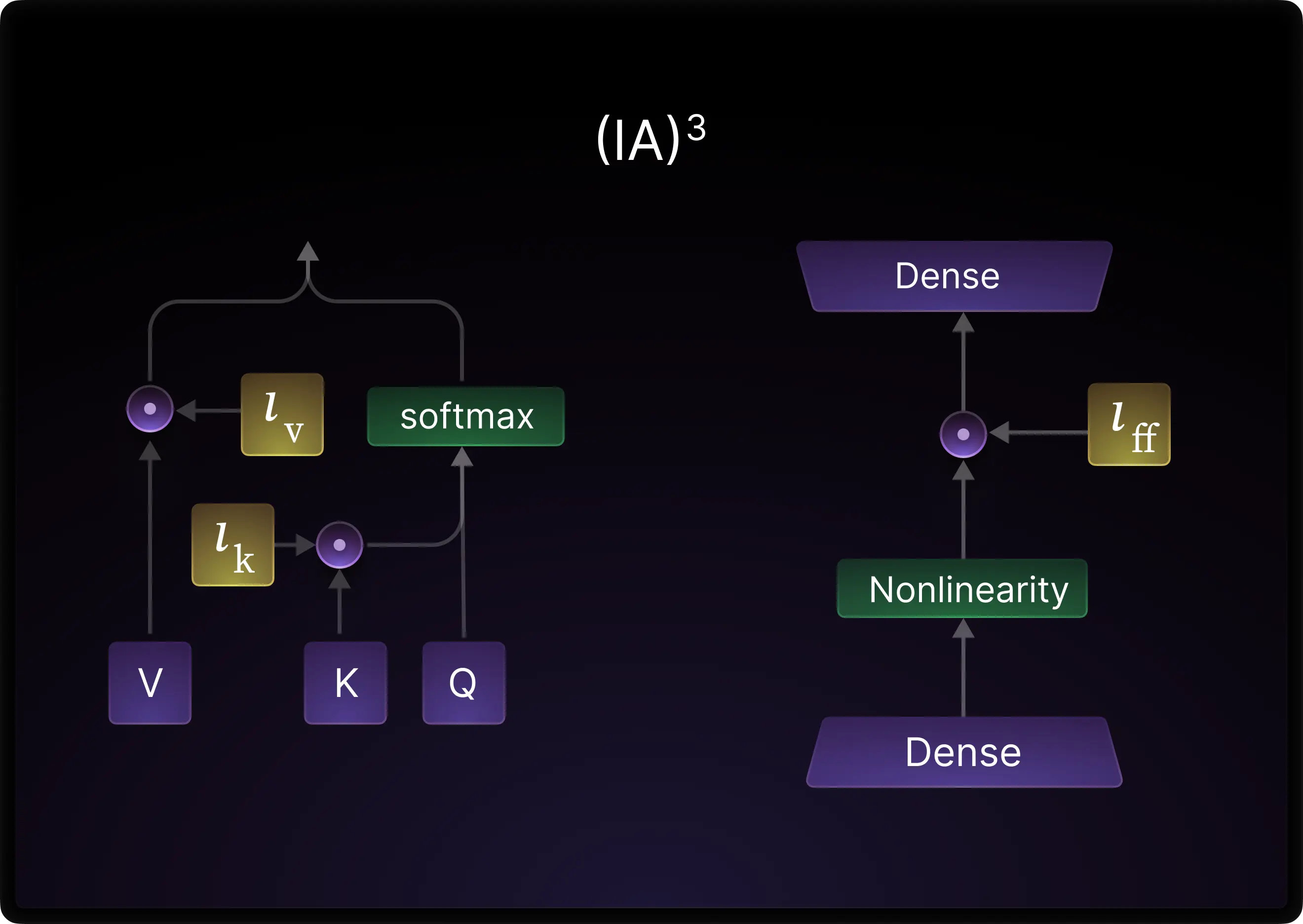
Overview of (IA)³, taken from the paper.

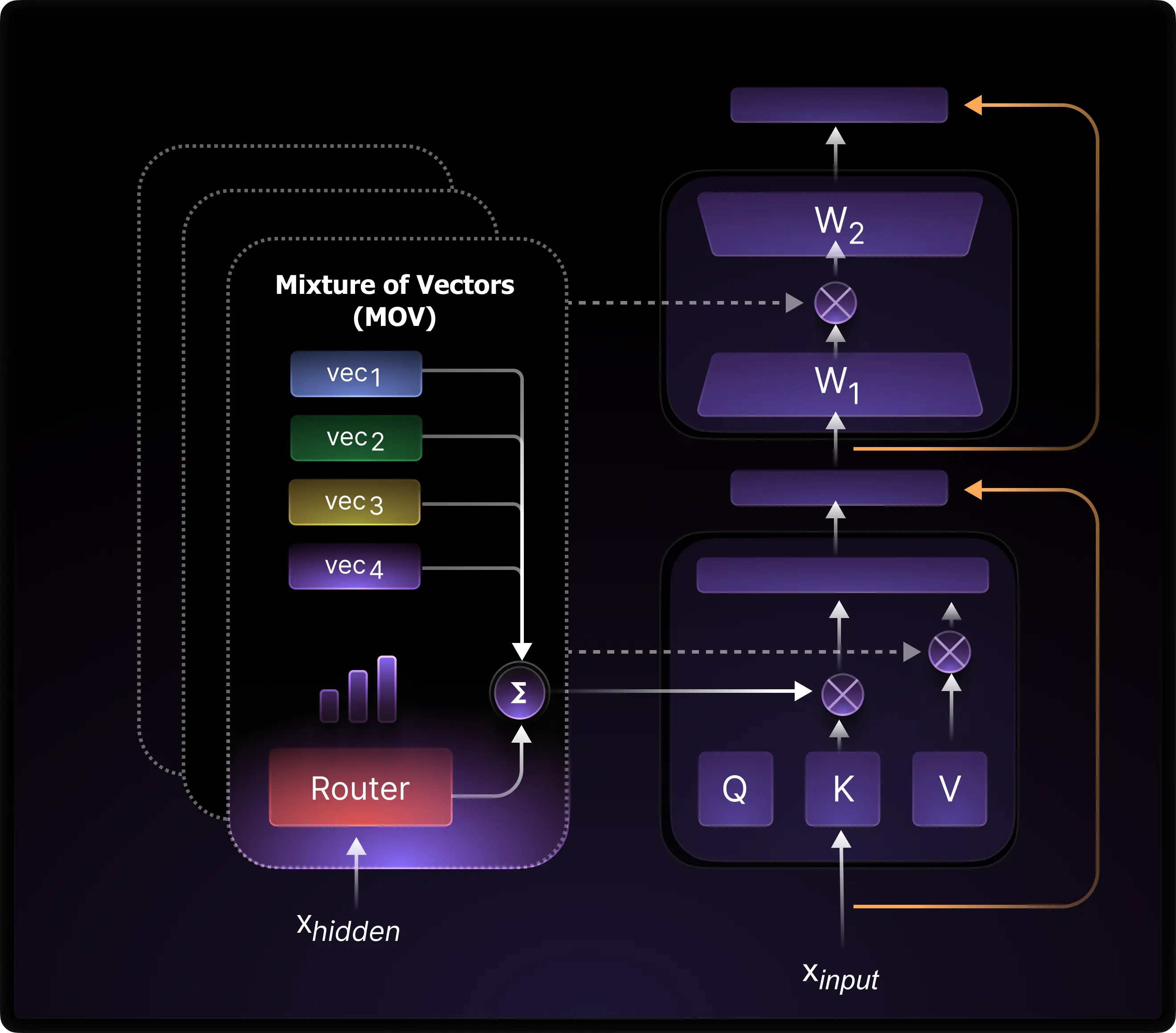
In Mixture of Vectors (MoV), the overall concept remains the same, but instead of learning one vector for each of the three tensors, we learn \(n\) (no. of experts) of them and combine them through a routing mechanism. The diagram below from the paper, gives an overview of this.

Implementation

Next, we will guide you through the implementation of the MoV and Router layers essential for this methodology. Additionally, we’ll discuss adapting these to fine-tune the LLaMA-2 model.

Router

A router is a linear layer that selects which experts to send the input towards. In MoV, the router is combined with the output from our experts, which are (IA)³ modules, and allows for conditional computation instead of using all of our parameters.

class Router(nn.Module):
    def __init__(self, input_dim, num_experts):
        super().__init__()
        self.ff = nn.Linear(input_dim, num_experts)
    def forward(self, x):
        logits = self.ff(x)
        probs = F.softmax(logits, dim=-1)
        return logits, probs

First, we define a linear layer that takes in the original input dimension and outputs a tensor with the corresponding number of experts. In the forward call, we first compute the logits with our dense layer and also return our probabilities from a softmax.

MoV Layer

The MoV layer combines the probabilities of the router network along with the outputs of each expert, which is an (IA)³ vector. We are computing the following equation, where \(s_i\) is the routing probability of the current expert, x is the token representation, and \(E_i\) is the current (IA)³ vector’s output:

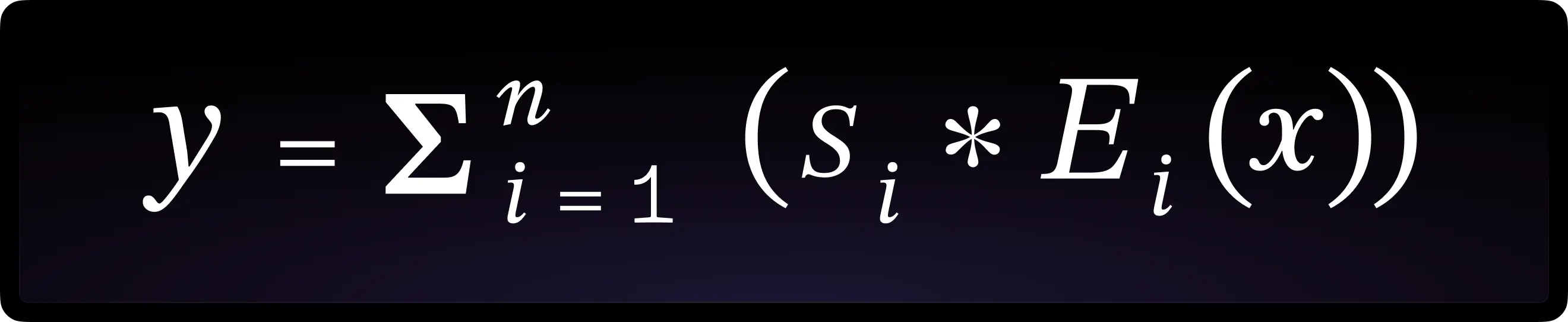
Although we can also implement Top-k routing, where we zero out the non-selected experts, the authors found that soft merging, which is a “weighted average of all experts computed within a specific routing block”, performed the best.

class MoV(nn.Module):
    def __init__(self, linear_layer, num_experts):
        super(MoV, self).__init__()
        # Original linear layer
        self.original_layer = linear_layer
        self.router = Router(self.original_layer.in_features, num_experts)
        self.experts = nn.Parameter(torch.ones(num_experts, linear_layer.out_features))
    def prepare_model_gradients(self):
        self.experts.requires_grad_(True)
        self.router.ff.weight.requires_grad_(True)
    def forward(self, x):
        frozen_output = self.original_layer(x)
        _, gating_probs = self.router(x)
        # Compute the weighted sum of expert outputs
        mov_combined = torch.einsum("bse,ed->bsd", gating_probs, self.experts)
        return frozen_output * mov_combined

To implement the MoV layer, we first store the original linear layer along with initializing the Router layer from the previous section and the experts, which are (IA)³ vectors. In the forward pass, we first compute the original output representation and then router probabilities. Afterward, we compute the weighted sum of the expert outputs along with the gating probabilities and rescale the original output. We also provide a prepare_model_gradients() method to set these tunable parameters and freeze the rest of the model in the next part.

Adding MoV to LLaMA-2

We stepped through the implementation specifics, but to get these layers integrated into an actual model, we need to iterate through the entire pretrained LLM and selectively apply theses MoV layers. For our experiments, we use the AutoModelForCausalLM on the Llama-2 decoder-only models.

def adapt_model_with_moe_peft(model, experts):
    # Only modify the key/value and linear activations
    llama_regex_match = "(.*(self_attn|LlamaAttention).(k_proj|v_proj).weight)|(.*LlamaMLP.down_proj.weight)"
    
    for n, _ in model.named_parameters():
        if re.search(regex_match, n) is None:
            continue
        # Get module that the parameter belongs to
        module_name = ".".join(n.split(".")[:-1])
        module = attrgetter(module_name)(model)
        module_parent_name = ".".join(n.split(".")[:-2])
        module_key_name = n.split(".")[-2]
        module_parent = attrgetter(module_parent_name)(model)
        setattr(module_parent, module_key_name, MoV(module, experts))

    # Freeze base model and set MoV weights as tunable
    for m in model.modules():
        m.requires_grad_(False)
        if isinstance(m, MoV):
            m.prepare_model_gradients()

When we print the model object, which is a Llama-2-7B model, we can see the defined embedding, 32 decoder layers, and language modeling head. Diving into the decoder, each layer consists of a self-attention layer, a multi-layer perceptron, input normalization, and a post-attention normalization. First, we define a regex to match the (IA)³ implementation where the parameters of the query/key and linear activations are modified. Then, we iterate through the model’s layers to find the valid parameters to inject our MoV layer. Finally, we need to freeze the base model and set the MoV layers as tunable, excluding the original layer. Note that using one expert is equivalent to applying (IA)³.

There are other tricks to improve our training efficiency, such as gradient checkpointing or mixed-precision training. After we add these trainable MoV layers into the decoder model, we can calculate the total number of parameters being tuned. With Llama-2 model, we get:

Note that using 1/10/20/60 expert(s) modifies less than 0.001%/0.01%/0.02%/0.05% of the total parameters, respectively. This is still incredibly memory efficient!

Experiments

We evaluate across 4 different datasets:

• The ScienceQA dataset is generated from elementary and high school multiple choice questions, where we select around 6000 samples (see our blog How to Fine-Tune GPT-3.5 Turbo With OpenAI API for more on fine-tuning with this dataset).

• Corpus of Linguistic Acceptability (CoLA) uses 23 linguistics publications to evaluate grammaticality with around 10000 samples. 

• Microsoft Research Paraphrase Corpus (MRPC) uses newswire articles and checks whether the sentence pairs are or are not paraphrases with 5000 pairs.

• Recognizing Textual Entailment (RTE) uses news and Wikipedia text for textual entailment, where we are given a premise and hypothesis and evaluate whether these texts logically follow (entail) or do not, with around 3000 samples.

All of our listed experiments use the Llama-2-7b model with the MoV technique. For our MoV runs, we default the learning rate to 2e-4 and run for 10 epochs. For full-tuning, we use a learning rate of 3e-5 and 5 epochs. In addition, we select the checkpoint that corresponds to the lowest validation loss. For evaluation, we use exact string match accuracy across the gold label and prediction.

 

From our results, we observe that using the MoE PEFT method consistently outperforms PEFT with an average four percent delta. Additionally, in some scenarios, such as with MRPC and RTE, MoV is equal or better than full-tuning our model. Lastly, we should note that increasing the number of experts does not always translate to better downstream performance. For example, Science QA and MRPC increase in performance as we scale from 1 to 60 experts, noting that this task can have even more experts. Both CoLA and RTE drop in performance after the 20th and 10th expert, respectively.

We recommend carefully tuning the number of experts while being mindful of the memory overhead. These trends are similarly observed by the authors. In addition, we can empirically state from our results that MoE PEFT helps close the gap between PEFT methods and full-tuning across both encoder-decoder and decoder-only models.

Conclusion

The MoE PEFT methods have great empirical benefits while being extremely memory effective. We are excited to further experiment with these methods along with providing a working implementation of MoV with Llama-2 models for anyone to try!

As we continue to test more methods, we will add what works best with LLMs to llm-engine so stay tuned for new changes that you can experiment with on your own! We also incorporate these methods into our Enterprise Generative AI Platform (EGP) and work with customers to fine-tune models for their unique use cases, implement cutting-edge retrieval augmented generation, and help them implement Generative AI Applications. We will continue to incorporate the latest research and techniques into our open-source packages, products, and processes as we help organizations unlock the value of AI.