Imagine you have submitted a research paper to a leading conference in the field of AI. Several reviewers will assess your work, each providing a rating from a set of four categories: accept, weak accept, weak reject, and reject. These ratings will play a crucial role in determining whether your work will eventually be accepted or rejected. Ideally, all reviewers should give the same rating, indicating they are applying the rating criteria consistently. However, in practice, their ratings may vary due to their interpretations of the paper's motivation, implementation, and presentation.

To evaluate the variability in rates and ensure a consistent rating process, the concept of inter-rater reliability (IRR) comes into play. Inter-rater reliability refers to statistical metrics designed to measure the level of observed agreement while controlling for agreement by chance. These metrics have also been called inter-rater agreement, inter-rater concordance, inter-coder reliability, and other similar names. Inter-rater reliability is a crucial metric for data collection in many domains that require rater consistency. When observing a high inter-rater reliability, raters are interchangeable because the ratings are similar regardless of who gives them. When observing a low inter-rater reliability, rates vary by individuals to a certain degree. This could result from factors like poorly calibrated raters, vague rating definitions, subjectivity or inherently indeterminate in their ratings.

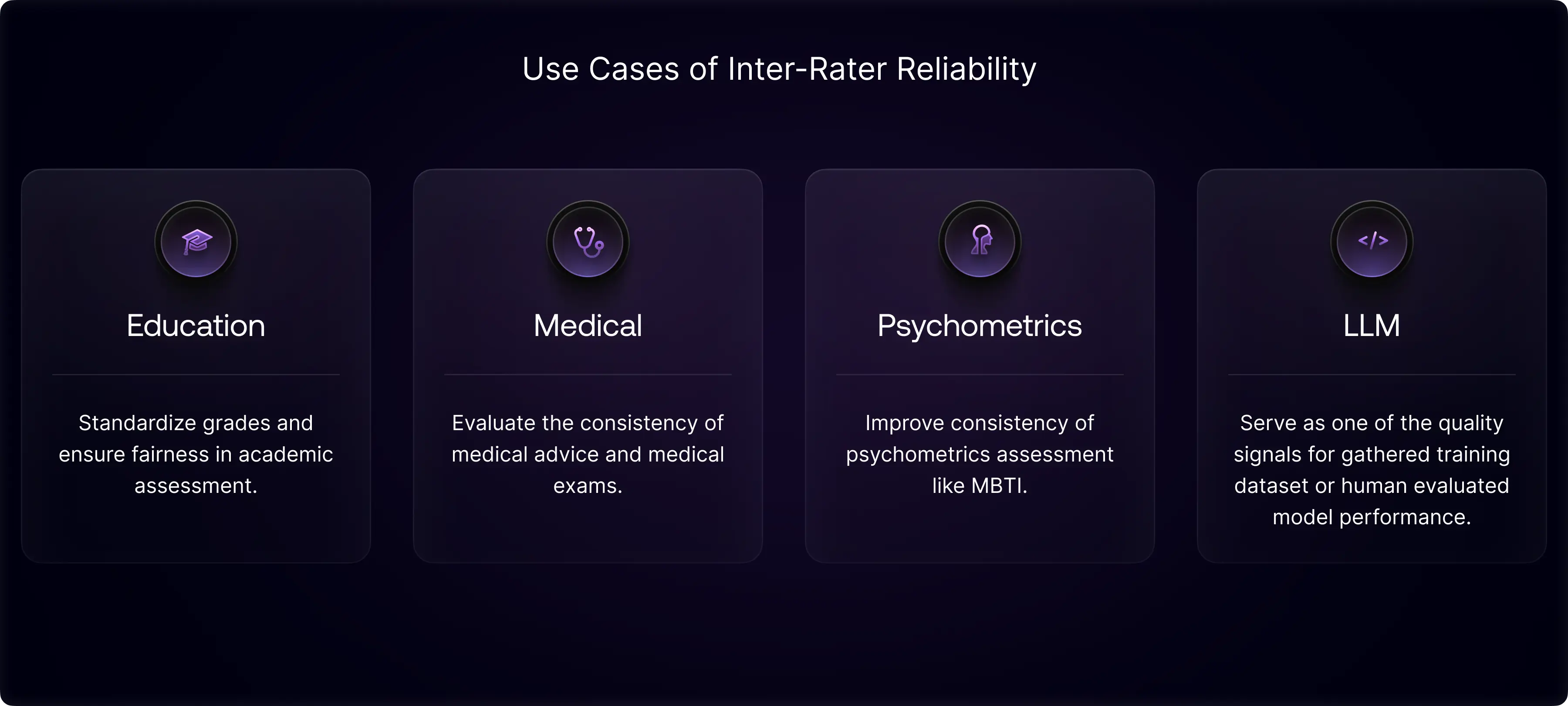
Inter-rater reliability is useful beyond paper reviews to fields like education, medical diagnosis, and psychometrics. It has also recently become a crucial tool in the development of large language models, primarily as a metric for estimating the quality of training data and assessing model performance. The wide range of applications showcases the extensive adaptability of inter-rater reliability. 

While IRR is a powerful statistical tool, it is not as well-known as related methods such as Pearson correlation, and it comes with its own complexities and nuances. This blog seeks to simplify the understanding of inter-rater reliability, offering easy-to-follow calculations and detailed explanations of its foundations. We'll begin with the fundamental concept of percentage agreement, then examine more intricate metrics, including Kappa coefficients and paradox-resistant coefficients. Topics such as validity coefficients and the role of inter-rater reliability in AI will also be discussed. We'll conclude by introducing how inter-rater reliability is employed in Scale’s quality evaluation system and the various initiatives undertaken to guarantee the utmost standard in data production.

Percentage Agreement

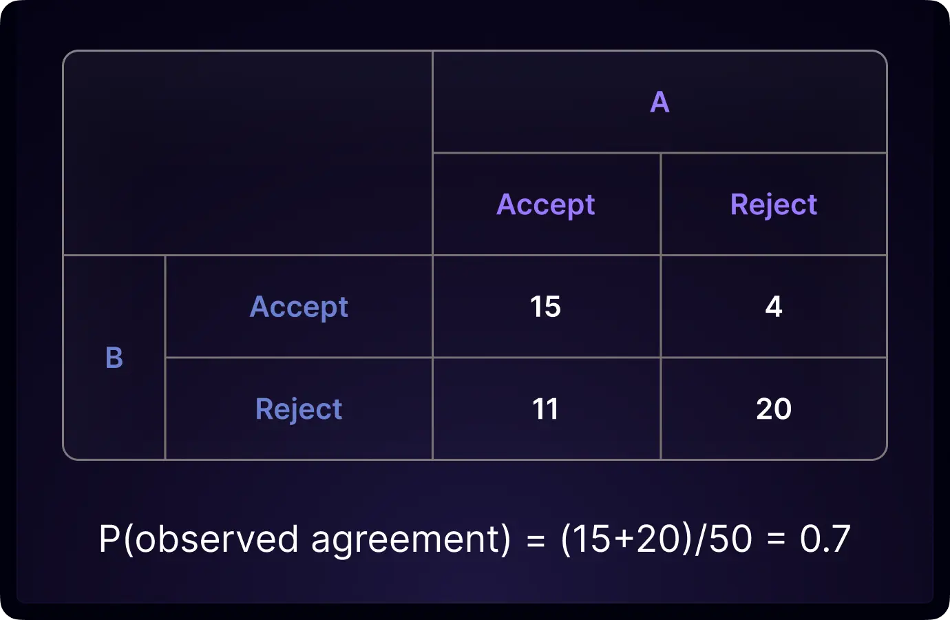
Let’s formulate a simple example to demonstrate metric calculation. Imagine we have 50 papers submitted to an AI conference and 2 raters (reviewers) to rate each subject (paper) as either accept or reject. The rating results are summarized in the table below. Both raters accepted the paper 15 times. Both raters rejected the paper 20 times. Rater A accepted and rater B rejected 11 times. Rater A rejected and rater B accepted 4 times.

If you need to assess how much two raters agree before knowing about IRR, a simple method is to look at how often the raters give the same ratings among all subjects. This approach is known as percentage agreement or observed percentage agreement. In our example, we determine the observed percentage agreement by calculating the fraction of subjects on which both raters agree, considering both accept and both reject, resulting in a value of 0.7. 

In contrast to the IRR metrics we discuss later, percentage agreement is easier to understand and visualize because it represents an actual percentage, not just as a number. For instance, in our example, a value of 0.7 translates to the two raters agreeing with each other 70% of the time.

Cohen’s Kappa

While observed percentage agreement is simple and easy to understand, it doesn’t account for the fact that raters could agree by random chance. Imagine a situation where each rater flipped a coin to decide whether to accept or reject each paper, two raters could agree to a considerable amount which would yield a positive observed percentage agreement.

In 1960, the statistician and psychologist Jacob Cohen, best known for his work in statistical power analysis and effect size, proposed the Kappa coefficient. Cohen’s Kappa uses an estimated percent chance agreement (denoted by Pₑ) to adjust the observed agreement (denoted by Pₐ). Cohen’s Kappa is calculated by comparing observed agreement Pₐ to the perfect agreement of 1 while deducting both by estimated chance agreement Pₑ. This formula has also evolved into a foundational framework for creating other inter-rater reliability metrics, establishing their range from negative infinity to 1.

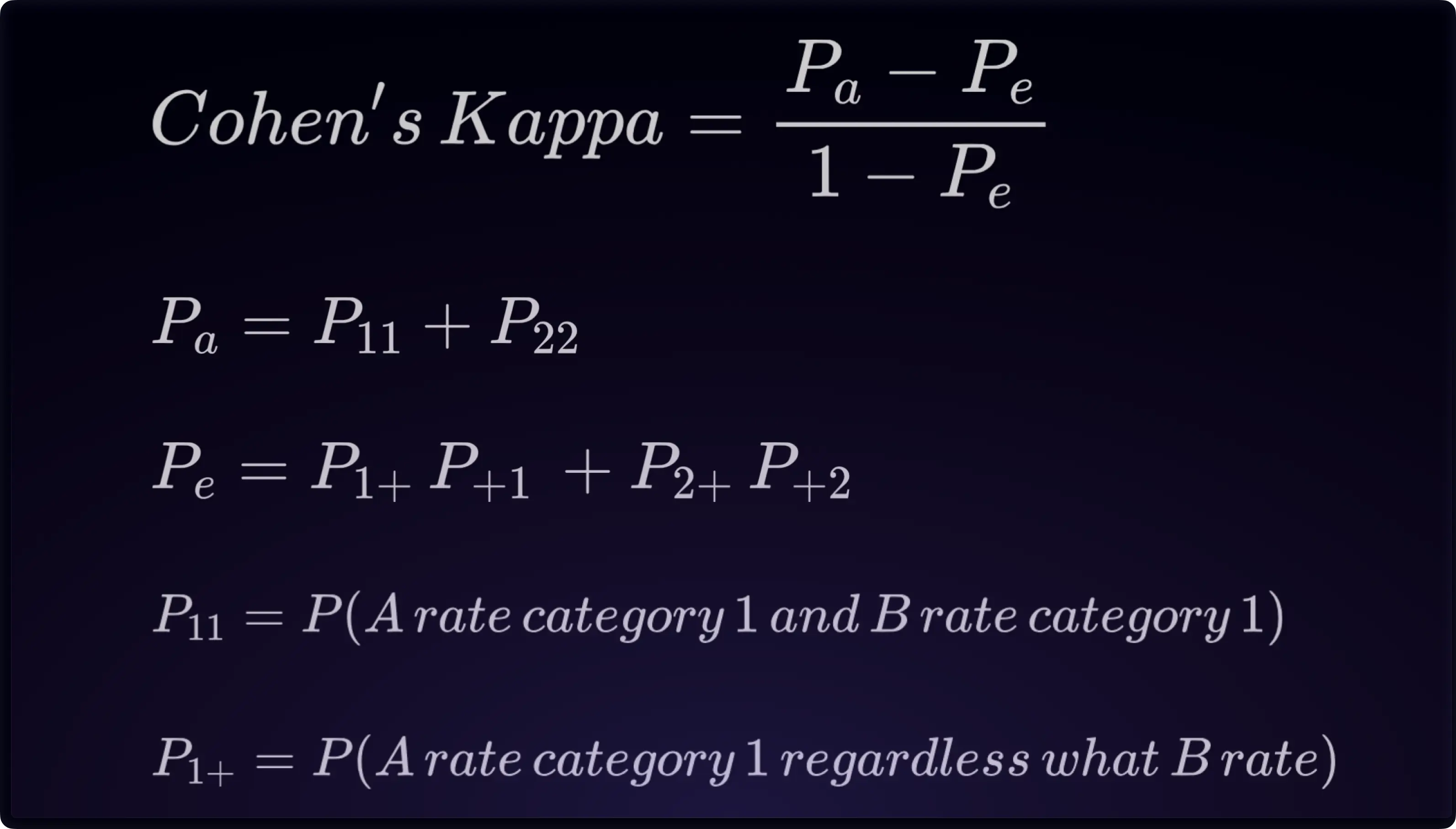
The calculation of the observed agreement Pₐ is performed in the same way as detailed in the previous chapter. In estimating percent chance agreement Pₑ, Cohen’s Kappa assumes that each rater randomly decides whether to accept or reject. It uses a rater’s observed marginal P(accept) as a rater’s propensity to accept. In our example, rater A accepted 26 papers and rejected 24 papers in total. Hence, its propensity to accept is assumed to be 26/50. On the other hand, A’s propensity to reject is 24/50. Similarly, the rater B’s propensity to accept is 19/50, and the propensity to reject is 31/50.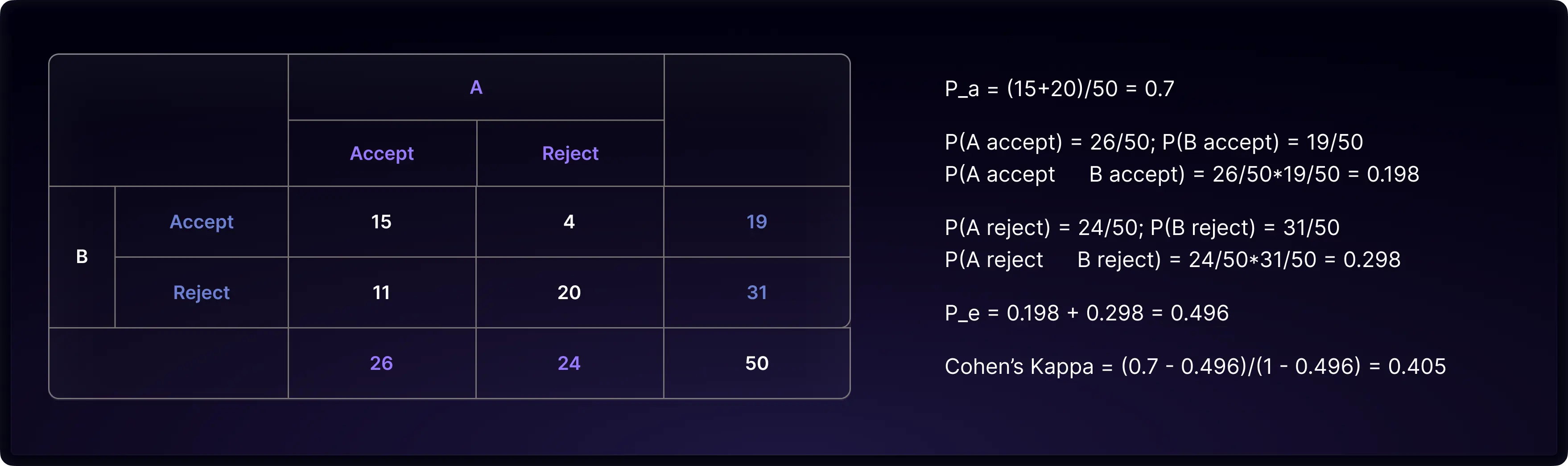

Cohen assumes each rater’s rating propensity is pre-determined before assessing the work. The estimated percentage chance agreement is the chance of two raters giving the same rate independently according to their rating propensity. Chance agreement could be either both raters accept a paper (A accept * B accept = 26/50 * 19/50) or both raters reject a paper (A reject * B reject = 24/50 * 31/50). The percentage chance agreement is the sum of two, which is 0.496. Finally, we apply the formula to calculate Cohen’s Kappa and get 0.405. 

Understanding Cohen's Kappa values, which range from negative infinity to 1, can be challenging. In 1977, Landis and Koch introduced a scale that categorizes Kappa values into specific levels of agreement, a system widely endorsed by researchers. According to this scale, values between (0.8, 1] suggest almost perfect agreement; (0.6, 0.8] suggest substantial agreement; (0.4, 0.6] suggest moderate agreement; (0.2, 0.4] suggest fair agreement; (0, 0.2] suggest slight agreement; and values less than 0 suggest poor agreement. For our example, a Cohen’s Kappa score of 0.405 falls into the category of moderate agreement. 

Fleiss’ Kappa & Krippendorff's Alpha

While Cohen's Kappa effectively measures 2-rater agreement, it is not designed for situations where there are multiple raters assessing the subjects. When involving multiple raters, agreement or disagreement is no longer binary. For example, with three raters, you could have two raters assigning the same rating while one assigns a different rating. This situation doesn't represent complete agreement or disagreement. Instead, the notion of agreement transforms into a spectrum.

In 1971, Joseph L. Fleiss, a distinguished statistician, built upon the groundbreaking work of Jacob Cohen by introducing an improved form of the Kappa coefficient. Named Fleiss' Kappa, this version expanded Cohen's original concept to effectively handle situations with multiple raters. Fleiss' Kappa is derived by applying the general formula that adjusts for chance agreement, leveraging Pₐ and Pₑ. Comprehending Fleiss’ Kappa hinges on understanding the calculation of these two parameters. 

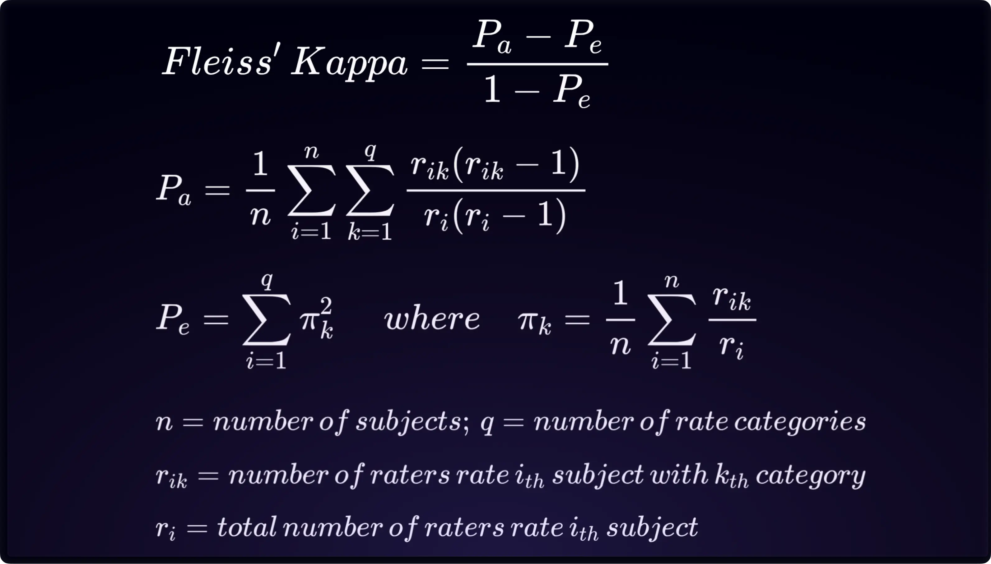
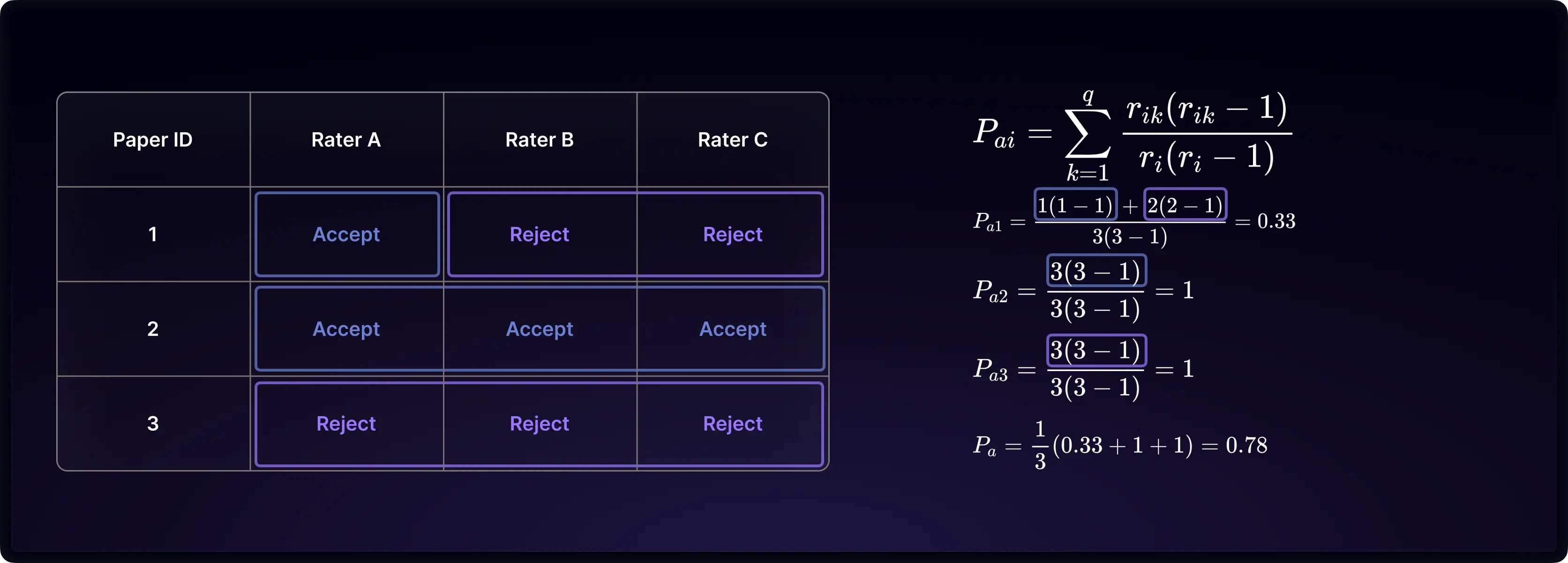
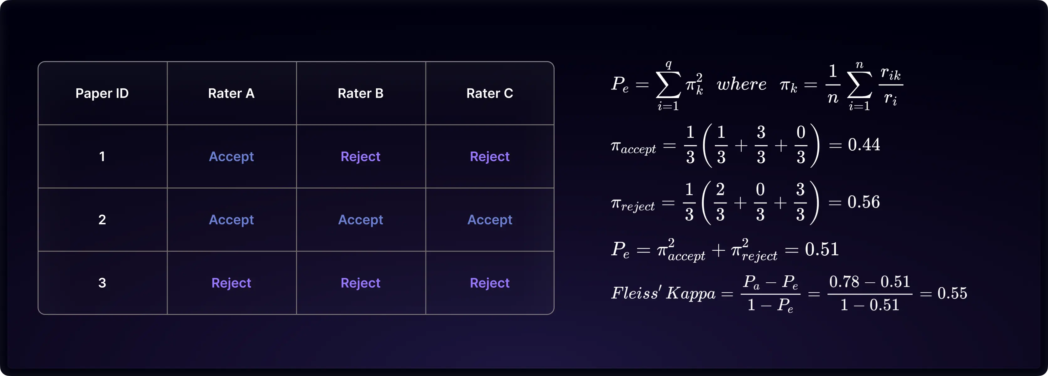
Consider an example with 3 raters reviewing 3 subjects, choosing between ‘accept’ or ‘reject’. The observed percentage agreement, Pₐ, is calculated by determining the proportion of agreeing rater pairs out of all possible pairs for each subject, then averaging these proportions across all subjects. In our example, each subject has three rater pairs (AB, AC, BC), and we calculate the agreeing proportion as the observed agreement for each subject. Then we average these proportions to obtain an overall Pₐ.

To estimate the percentage chance agreement (Pₑ), Fleiss' Kappa assumes that a rater's choice of a particular rating equals the overall observed rate of that rating in the data. This method simplifies the problem by assuming uniform rate propensity across all raters, making Pₑ a measure of how often two raters would randomly agree independently. By inserting both Pₐ and Pₑ into the chance adjustment formula, the value of Fleiss' Kappa is derived.

Krippendorff's Alpha, developed by Klaus Krippendorff, is another popular measure of inter-rater reliability that shares a foundational similarity with Fleiss' Kappa. Generally, Krippendorff's Alpha tends to produce results that are close to those obtained from Fleiss' Kappa. The primary distinction of Krippendorff's Alpha lies in its capacity to accommodate scenarios with missing ratings, where not every rater evaluates each subject. Furthermore, it incorporates subject size correction terms, which lead to more conservative estimations, particularly when the number of raters falls below five.

Level of Measurement

In our example of paper review, there are two rating categories: 'accept' and 'reject.' These categories are distinct and do not intersect. In this case, the rating's level of measurement is classified as nominal, where 'accept' and 'reject' form a dichotomy. Different ratings represent complete disagreement.

If the rating categories are expanded to include 'accept', 'weak accept', 'weak reject', and 'reject', the level of measurement transitions to ordinal, reflecting an inherent order within the categories. This allows for the establishment of a hierarchical sequence from 'accept' through 'weak accept' and 'weak reject', to 'reject'. In this framework, 'weak accept' is perceived as a lower level of agreement with 'reject', rather than being a complete disagreement.

A specific subtype of the ordinal level of measurement is the interval level, characterized by equal distances between adjacent ratings. If the intervals between 'accept', 'weak accept', 'weak reject', and 'reject' are equal, our example could be classified as interval ratings. However, this might not be entirely appropriate as some may perceive the gap between 'weak accept' and 'weak reject' to be larger than the others, indicating a shift in the direction of the outcome. For a clearer understanding, the table below outlines the three levels of measurement we've covered, complete with relevant examples.

Level of Measurement	Characteristic	Example
Nominal	Ratings without inherent order.	Classifying diseases in medical diagnosis.
Ordinal	Ratings have a meaningful order, but intervals aren't consistent.	A 1-5 star rating in app stores, with 1 star typically indicating poor quality, significantly different from higher ratings.
Interval	Equal intervals between ratings.	IQ scores, where the difference between scores is designed to be consistent, indicating equal increments in intellectual ability.

To transition from nominal to other measurement levels, weights are applied to transform the binary framework of agreement or disagreement into varying degrees of agreement. Typically, an exact match in the rate category is assigned a weight of 1 and a partial match is assigned a weight below 1. The specific scale of these weights is dictated by the mathematical formulation used to measure the distance between ratings. For instance, the table below illustrates a linear weight approach, where the weight of agreement decreases linearly as the distance between ratings increases. Additionally, there are alternative weighting methods such as quadratic, ordinal, and more.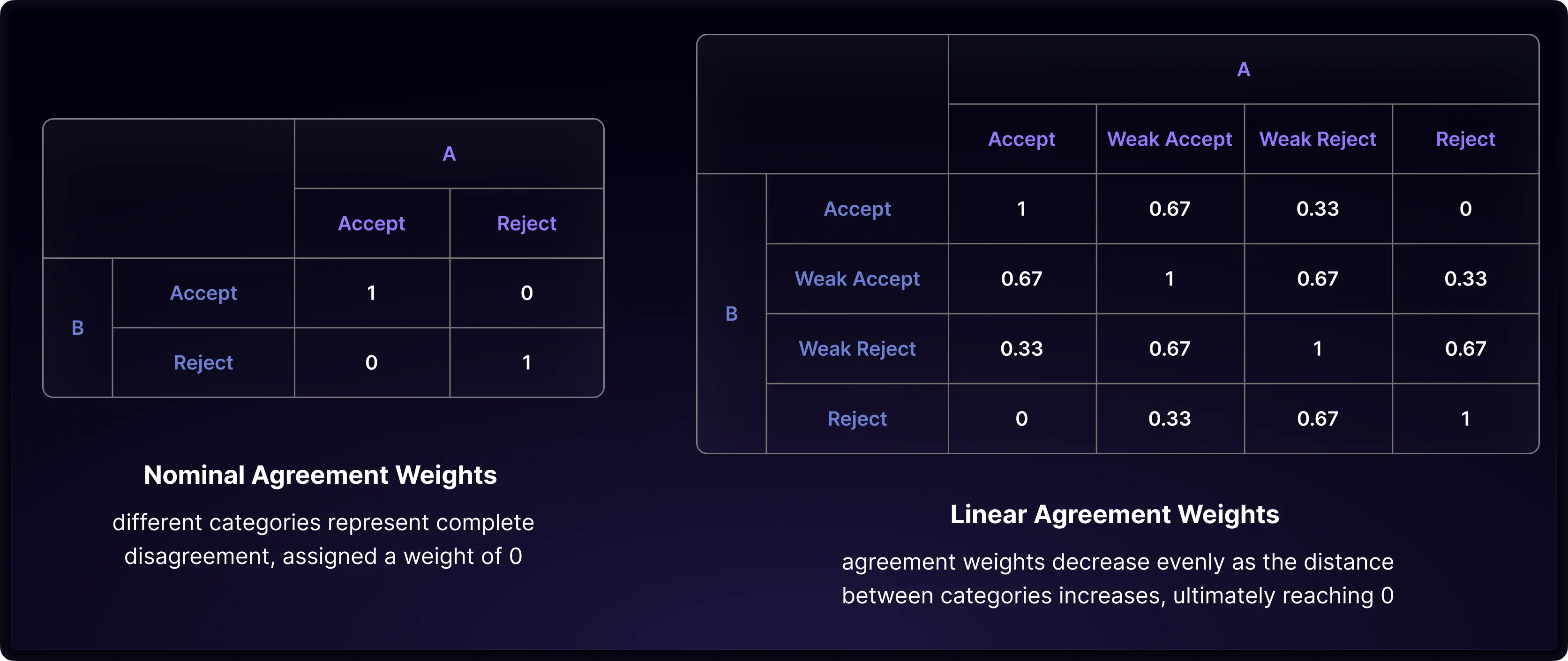

After selecting a weighting method, it should be consistently applied to both the observed percentage agreement (Pₐ) and the percentage chance agreement (Pₑ). Weighted Cohen’s Kappa, a variation of Cohen’s Kappa, incorporates these weights. As the field of inter-rater reliability evolves, incorporating weights has become a standard practice to encompass various levels of agreement in the metrics.

Kappa’s Paradox

While Kappa coefficients are designed to adjust for chance agreement in a straightforward manner, they can sometimes result in unexpectedly low values when compared to the observed percentage agreement (Pₐ). Take, for instance, a scenario where 10 cases of both 'accept' are shifted to both 'reject' in our 2-rater example. In this situation, Cohen’s Kappa significantly drops from 0.405 to 0.219, even though the observed agreement percentage remains constant at 0.7. 

This phenomenon, known as Kappa’s paradox, is primarily attributed to changes in the percentage chance agreement estimation. When the observed agreement of 0.7 is compared against a chance agreement of 0.496, it is seen as a good agreement, yielding a Cohen’s Kappa of 0.405. However, against a chance agreement of 0.616, the same observed agreement of 0.7 doesn't appear as strong, thus resulting in a lower Cohen’s Kappa of 0.219. Detailed calculations are presented in the illustration below.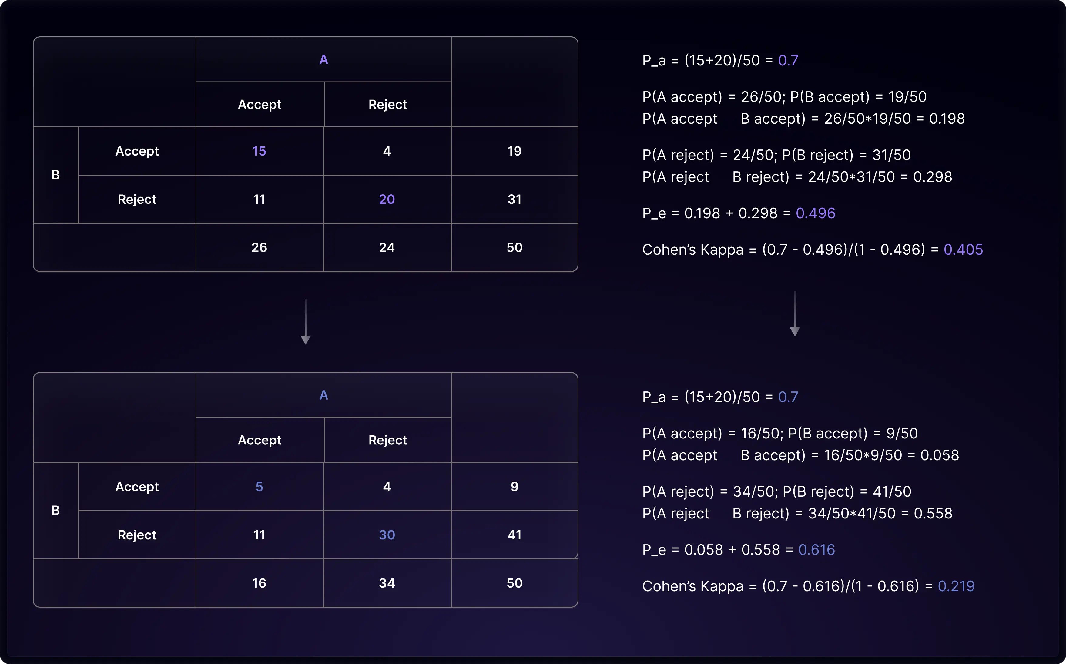 

Kappa's paradox becomes particularly evident when observed ratings are skewed towards one or a few categories. In such cases, the percentage of chance agreement is often larger than anticipated, due to the data skewness. This can result in a Cohen’s Kappa value that is near zero or even negative, suggesting that the level of agreement is no better than, or even worse than, what would be expected by random chance. This outcome is paradoxical and often counterintuitive, as it contradicts the consistency level many researchers would perceive under these situations.

One explanation of Kappa’s Paradox stems from its approach to estimating the percentage of chance agreement. Remember that Cohen’s Kappa presumes each rater has a certain propensity to rate in a particular way, even before engaging in the rating process. This chance agreement is calculated by considering each rater’s propensity as an independent event. However, there's a catch: the estimation of each rater’s propensity is derived from their observed ratings, which are influenced by the subjects they rate. This reliance on observed ratings compromises the assumption of independent rating, leading to an imperfect estimation of chance agreement. Kappa’s paradox isn't unique to Cohen’s Kappa; both Fleiss’s Kappa and Krippendorff's Alpha encounter similar issues, as they also use observed marginal probabilities to approximate a rater’s propensity.

Paradox-Resistant Coefficients

In 1981, Robert Brennan and Dale Prediger introduced an agreement coefficient, arguably the simplest among all chance-corrected coefficients aimed at resolving Kappa’s paradox. The Brennan-Prediger coefficient is based on the premise that a rater's likelihood of choosing any particular rating is uniformly distributed across all available categories. Therefore, if there are 𝒒 categories, the probability of a rater selecting any one category is 1/𝒒. With this uniform distribution assumption, the expected chance agreement between two raters is calculated as 𝒒×(1/𝒒)² = 1/𝒒. The diagram below contrasts the chance agreement observed in the previous example with the chance agreement calculated using the Brennan-Prediger coefficient.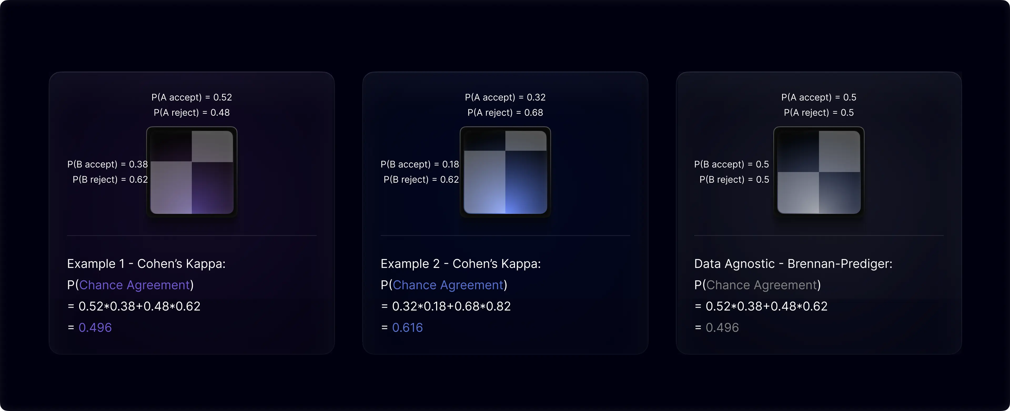

The Brennan-Prediger coefficient effectively circumvents Kappa’s paradox by consistently providing a constant level of chance agreement, regardless of whether the observed ratings are balanced or skewed. However, it is crucial to validate the assumption of uniform rating propensity when applying the Brennan-Prediger coefficient. In the context of our paper review example, a 50/50 propensity of accepting or rejecting seems more plausible if raters are strictly evaluating based on content criteria without any quotas for acceptance or rejection. Conversely, if a conference is known for its stringent acceptance rates and raters are subconsciously influenced to maintain a similar level of selectivity, then a 50/50 distribution would not be an accurate reflection of their rating propensity.

In 2008, Kilem Gwet developed a new agreement coefficient known as Gwet’s AC, specifically aimed at overcoming the challenges posed by Kappa’s paradox. Additionally, you may come across the terms AC₁ and AC₂ in this context, where AC₁ is used for nominal rating categories and AC₂ applies to other levels of measurement in ratings. 

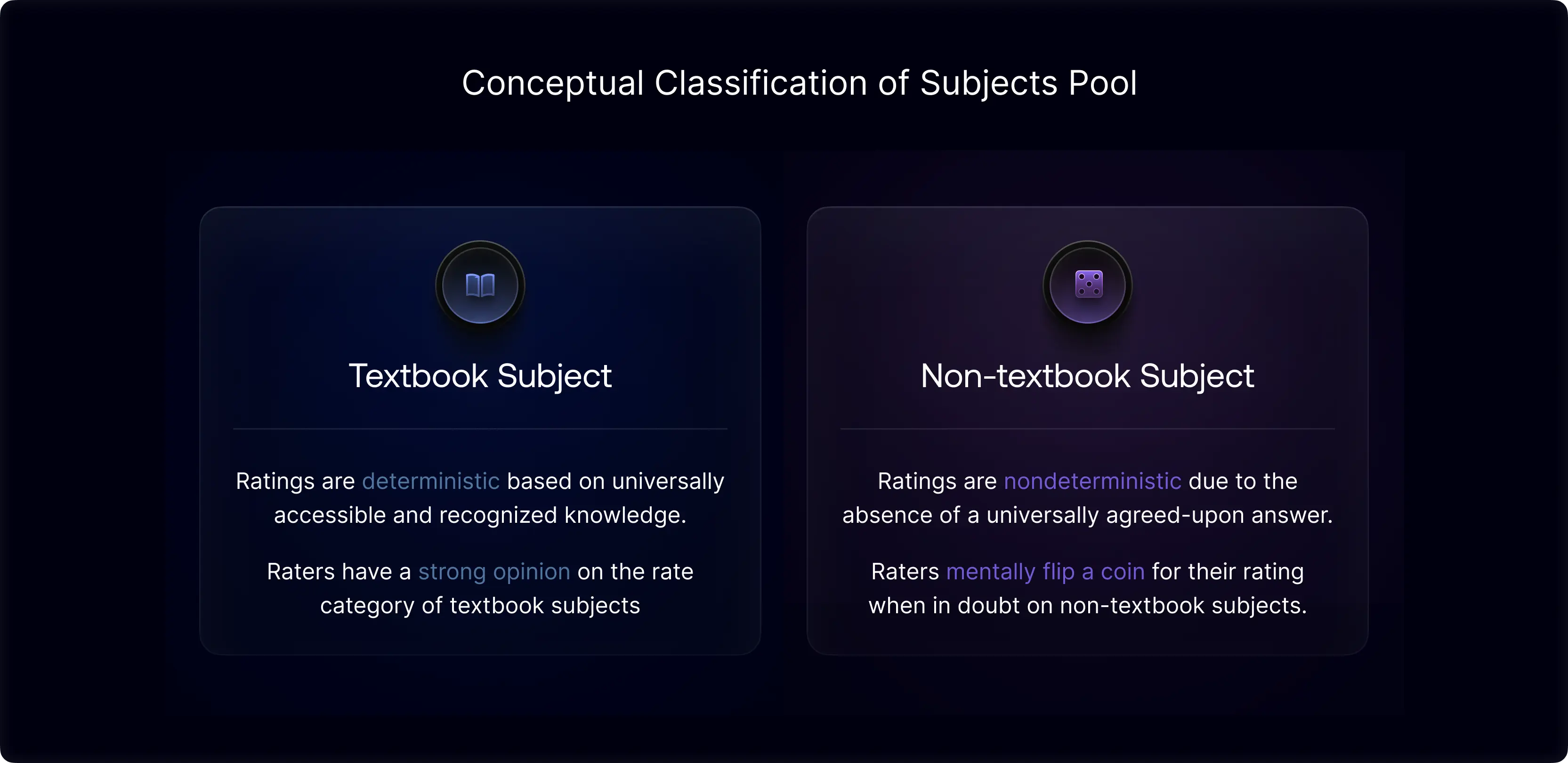
Gwet’s theory conceptually categorizes subjects into two distinct types: textbook and non-textbook. Textbook subjects have deterministic rating categories, determined by the universally accessible and understandable public knowledge. Non-textbook subjects, conversely, are marked by their non-deterministic nature, where even the collective knowledge of raters fails to provide definitive answers.  Non-textbook subjects could also involve subjective judgment, where ratings are shaped by individual preferences. Textbook subjects are often called 'easy-to-rate', while their non-textbook counterparts are called 'hard-to-rate' due to their inherent complexity. Gwet proposed that chance agreement is particularly relevant in non-textbook subjects, as these often involve raters making decisions based on personal opinions or selecting from multiple viable options at random.

Ideally, distinguishing between textbook and non-textbook subjects allows for a more precise calculation of chance agreement, especially in non-textbook subjects where greater randomness is expected. However, classifying subjects into these categories is not straightforward and demands extensive understanding of the domain knowledge related to the rating task. Gwet's approach involves estimating the probability of a subject being non-textbook based on the observed rate of disagreement, under the assumption that disagreements are more likely to occur in non-textbook cases. While the precise mathematical formulation of Gwet’s AC is complex and beyond the scope of this blog, a key takeaway is that data skewness towards a few ratings would reduce the likelihood of encountering non-textbook subjects. The underlying assumption is that hard-to-rate subjects are rare when most subjects are assigned into one rating category. This feature effectively constrains the level of chance agreement when ratings are skewed.

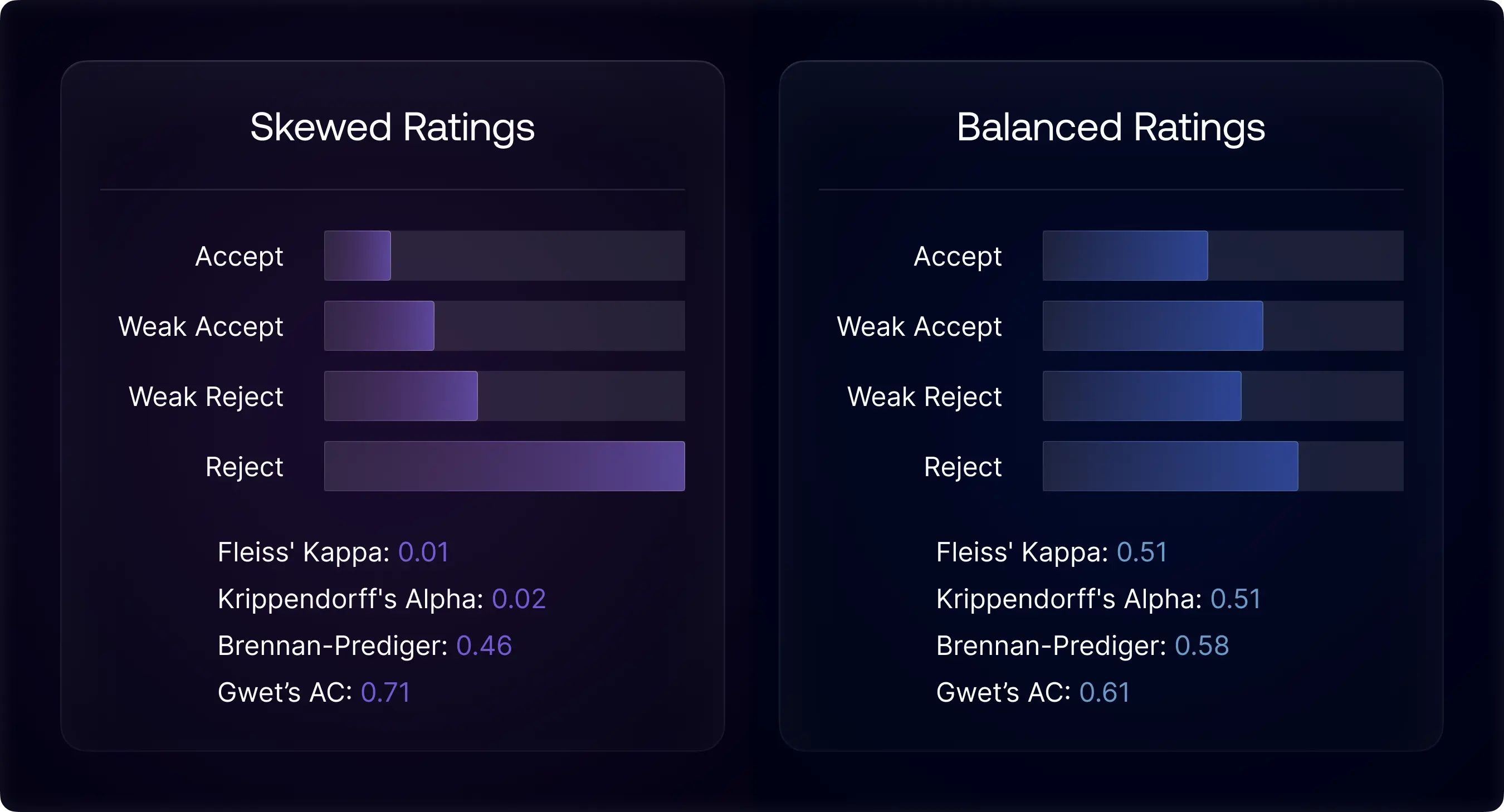
To mitigate Kappa’s paradox, another empirical strategy is diversifying the subject pool, although its suitability varies with the research context. Theoretically, a diverse subject pool across the rated dimension should result in balanced rating categories, thereby avoiding Kappa’s paradox. To demonstrate, we simulated two scenarios: one rating distribution predominantly featuring papers likely to be rejected and another with a more even mix of papers likely to be accepted or rejected. The results show that Kappa and paradox-resistant coefficients heavily diverge in the skewed scenario but align in the more balanced rating scenario. In practice, leveraging a set of inter-rater reliability metrics can achieve a more reliable agreement evaluation, adaptable to data distribution.

 

Related Topics In Practice

Inter-rater reliability is a crucial metric for assessing consistency in ratings, but it does not encompass the entirety of data quality assessment, particularly in the context of validity. When a 'true' rate category is identifiable, validity becomes a measure of the accuracy of ratings. It is important to recognize that reliability and validity may not always align, as consensus among raters doesn't guarantee correctness. Inter-rater reliability metrics can be adapted to only consider consensus on the 'true' category, thereby serving as a validity coefficient. Operationally, the determination of the 'true' rating category typically involves setting a clear definition and consulting experts for their assessments.

Validity isn't always applicable, particularly when a clear 'true' rate category is absent. For instance, in subjective scenarios like rating a fitness app, there's unlikely to be a universally correct rating due to personal preference. Without a definitive 'true' rate set by an operational definition, the concept of validity loses relevance. In such scenarios, it's practical to view raters as representing diverse segments of a larger population, which impacts the expectations and interpretations of inter-rater reliability. 

The metrics for inter-rater reliability we've discussed mainly apply to categorical data, often seen in classifications or Likert scale ratings. For continuous data, where ratings might include decimal points, intra-class correlation coefficients (ICC) are more suitable for assessing reliability. Continuous data introduces the possibility of random noise, as even well-aligned raters may have slight differences in their ratings. Intra-class correlation offers a framework to model variations due to the rater, the subject, and noise, providing input to calculate inter-rater reliability in such contexts.

In the field of AI and Large Language Model (LLM), inter-rater reliability is increasingly used, especially in evaluating human-annotated training datasets and in assessing human evaluations of model performance. Notable applications include Google's use of Krippendorff's Alpha for dataset assessment and Meta's use of Gwet’s AC in model performance evaluation. In our research on published studies, we generally observed a higher inter-rater reliability in dataset annotation than in model evaluation. This is likely attributed to the increased subjectivity inherent in the model evaluation process. Furthermore, difficulty in rating a subject might impact IRR, as Anthropic observed that more sophisticated topics get lower agreement. There's also a growing call in the research community to disclose data collection specifics and IRR measures, as they shed light on data quality and subject difficulty, offering valuable insights for other researchers.

We have also witnessed innovative applications of IRR beyond data annotation and model evaluation. For instance, Stability AI employed rater engagement and IRR in choosing between various user interface and rate category designs for their web application, leading to more data collected with higher agreement. Moreover, a Stanford research utilized IRR to understand the alignment between human and language model, particularly in when to initiate grounding actions in a conversation. These expanding applications indicate a growing importance of inter-rater reliability in the ongoing development of AI.

Summary

Hopefully this blog has offered a clear and engaging look into the world of inter-rater reliability. Next time you're involved in academic submissions or peer reviews, you might have a deeper understanding on how ratings influence final outcomes and the role of inter-rater reliability. Here are some key takeaways:

• Inter-rater reliability quantifies agreement among independent raters who rate, annotate, or assess the same subject.

• Inter-rater reliability is a statistical tool designed to correct for chance agreement. It is applicable in multi-rater contexts and flexible across diverse levels of measurement.

• Be cautious about Kappa’s paradox in cases of skewed rating distributions. Consider using both Kappa coefficients and paradox-resistance coefficients for a robust evaluation.

• Agreement doesn't inherently imply accuracy. Validity measurement is essential alongside reliability when a definitive 'true' rating category exists and can be clearly identified.

• The field of AI is increasingly adopting inter-rater reliability, particularly for assessing human-annotated training data and evaluating model performance.

At Scale, we have created a system for evaluating data production quality that integrates various indicators of quality. We assess the consistency of ratings using IRR, ensuring alignment with our anticipated standards, which vary based on the level of subjectivity of the rating task. We utilize 'golden' tasks, which are rated by experts, to ensure the validity of the data and to guardrail the competency of the data contributors. We perform linguistic analysis to measure the data's diversity in various aspects. We also use machine learning to assess raters' adherence to guidelines and their writing abilities, and to create tools for correcting grammar and syntax errors during annotation. By combining and validating these different quality signals, we establish a comprehensive and dependable system for assessing data quality.

Scale’s commitment to quality doesn't end with evaluation. We proactively apply insights from quality evaluations by regularly enhancing our rater training programs, making rating categories clearer, and engaging top professionals in data contribution. These combined efforts reflect Scale’s dedication to upholding exceptional data quality standards, ensuring we deliver superior data for advanced AI applications.

Looking ahead, Scale remains deeply invested in research and innovation with statistical methods to ensure the highest quality standards for our products and services. As we continue to push the boundaries of quality evaluation systems, we invite you to collaborate with us on this journey to power the world’s most advanced LLMs. 

Contact our sales team to explore how Scale’s Data Engine can help accelerate your data strategy.

—

A special thanks to the individuals below for their insightful feedback and suggestions for this blog post.

Scale AI: Dylan Slack, Russell Kaplan, Summer Yue, Vijay Karunamurthy, Lucas Bunzel

External: David Stutz, David Dohan